10th DIMACS Implementation Challenge:

http://www.cc.gatech.edu/dimacs10/index.shtml

As stated on their main website (
http://dimacs.rutgers.edu/Challenges/ ), the "DIMACS Implementation
Challenges address questions of determining realistic algorithm
performance where worst case analysis is overly pessimistic and
probabilistic models are too unrealistic: experimentation can provide
guides to realistic algorithm performance where analysis fails."

For the 10th DIMACS Implementation Challenge, the two related
problems of graph partitioning and graph clustering were chosen.
Graph partitioning and graph clustering are among the aforementioned
questions or problem areas where theoretical and practical results
deviate significantly from each other, so that experimental outcomes
are of particular interest.

Problem Motivation

Graph partitioning and graph clustering are ubiquitous subtasks in
many application areas. Generally speaking, both techniques aim at
the identification of vertex subsets with many internal and few
external edges. To name only a few, problems addressed by graph
partitioning and graph clustering algorithms are:

    * What are the communities within an (online) social network?
    * How do I speed up a numerical simulation by mapping it
        efficiently onto a parallel computer?
    * How must components be organized on a computer chip such that
        they can communicate efficiently with each other?
    * What are the segments of a digital image?
    * Which functions are certain genes (most likely) responsible
        for?

Challenge Goals

    * One goal of this Challenge is to create a reproducible picture
        of the state-of-the-art in the area of graph partitioning
        (GP) and graph clustering (GC) algorithms. To this end we
        are identifying a standard set of benchmark instances and
        generators.

    * Moreover, after initiating a discussion with the community, we
        would like to establish the most appropriate problem
        formulations and objective functions for a variety of
        applications.

    * Another goal is to enable current researchers to compare their
        codes with each other, in hopes of identifying the most
        effective algorithmic innovations that have been proposed.

    * The final goal is to publish proceedings containing results
        presented at the Challenge workshop, and a book containing
        the best of the proceedings papers.

Problems Addressed

The precise problem formulations need to be established in the course
of the Challenge. The descriptions below serve as a starting point.

    * Graph partitioning:

      The most common formulation of the graph partitioning problem
      for an undirected graph G = (V,E) asks for a division of V into
      k pairwise disjoint subsets (partitions) such that all
      partitions are of approximately equal size and the edge-cut,
      i.e., the total number of edges having their incident nodes in
      different subdomains, is minimized. The problem is known to be
      NP-hard.

    * Graph clustering:

      Clustering is an important tool for investigating the
      structural properties of data. Generally speaking, clustering
      refers to the grouping of objects such that objects in the same
      cluster are more similar to each other than to objects of
      different clusters. The similarity measure depends on the
      underlying application. Clustering graphs usually refers to the
      identification of vertex subsets (clusters) that have
      significantly more internal edges (to vertices of the same
      cluster) than external ones (to vertices of another cluster).

There are 10 data sets in the DIMACS10 collection:

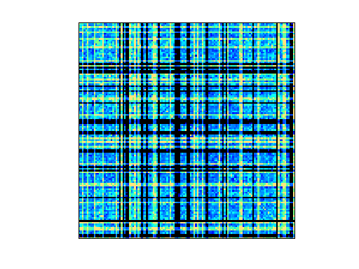
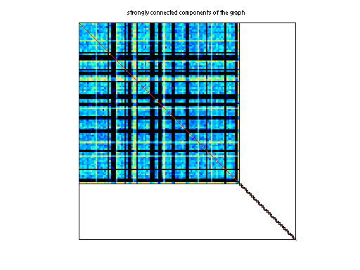
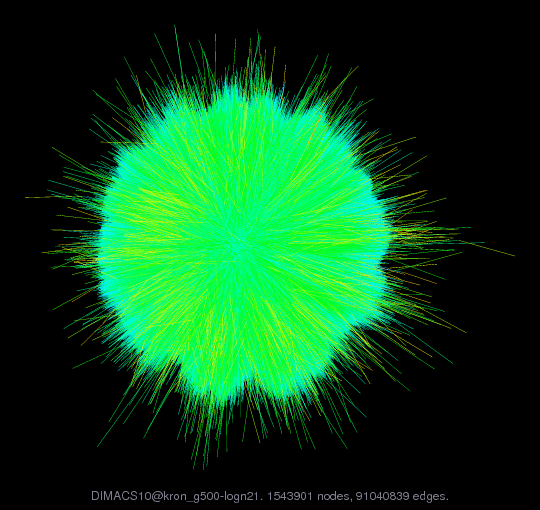
Kronecker:  synthetic graphs from the Graph500 benchmark
dyn-frames: frames from a 2D dynamic simulation
Delaunay:   Delaunay triangulations of random points in the plane
coauthor:   citation and co-author networks
streets:    real-world street networks
Walshaw:    Chris Walshaw's graph partitioning archive
matrix:     graphs from the UF collection (not added here)
random:     random geometric graphs (random points in the unit square)
clustering: real-world graphs commonly used as benchmarks
numerical:  graphs from numerical simulation

Some of the graphs already exist in the UF Collection.  In some cases,
the original graph is unsymmetric, with values, whereas the DIMACS
graph is the symmetrized pattern of A+A'.  Rather than add duplicate
patterns to the UF Collection, a MATLAB script is provided at
http://www.cise.ufl.edu/research/sparse/dimacs10 which downloads
each matrix from the UF Collection via UFget, and then performs whatever
operation is required to convert the matrix to the DIMACS graph problem.
Also posted at that page is a MATLAB code (metis_graph) for reading the
DIMACS *.graph files into MATLAB.


Kronecker:  Kronecker Generator Graphs

The original Kronecker files contain self-loops and multiple edges.
These properties are also present in real-world data sets. However,
some tools cannot handle these "artifacts" at the moment. That is why
we present "cleansed" versions of the data sets as well.  For the
Challenge you should expect to be confronted with the original data
with self-loops and multiple edges. However, the final decision on
this issue will be made based on participant feedback.

All files have been generated with the R-MAT parameters A=0.57, B=0.19,
C=0.19, and D=1-(A+B+C)=0.05 and edgefactor=48, i.e., the number of
edges equals 48*n, where n is the number of vertices. Details about the
generator and the parameter meanings can be found on the Graph500
website.  ( http://www.graph500.org/Specifications.html )

There are 12 graphs in the DIMACS10 test set at
http://www.cc.gatech.edu/dimacs10/index.shtml .  Them come in 6 pairs.
One graph in each pair is a multigraph, with self-edges.  The other
graph is the nonzero pattern of the first (binary), with self-edges
removed.  MATLAB cannot directly represent multigraph, so in the UF
Collection the unweighted multigraph G is represented as a matrix A
where A(i,j) is an integer equal to the number edges (i,j) in G.

The binary graphs include the word 'simple' in their
name In the UF Collection, only the multigraph is included,
since the simple graph can be constructed from the multigraph.
If A is the multigraph, the simple graph S can be computed as:

   S = spones (tril (A,-1)) + spones (triu (A,1)) ;

DIMACS10 graph:                        UF matrix:
---------------                        -------------
kronecker/kron_g500-logn16             DIMACS10/kron_g500-logn16
kronecker/kron_g500-simple-logn16

kronecker/kron_g500-logn17             DIMACS10/kron_g500-logn17
kronecker/kron_g500-simple-logn17

kronecker/kron_g500-logn18             DIMACS10/kron_g500-logn18
kronecker/kron_g500-simple-logn18

kronecker/kron_g500-logn19             DIMACS10/kron_g500-logn19
kronecker/kron_g500-simple-logn19

kronecker/kron_g500-logn20             DIMACS10/kron_g500-logn20
kronecker/kron_g500-simple-logn20

kronecker/kron_g500-logn21             DIMACS10/kron_g500-logn21
kronecker/kron_g500-simple-logn21


References: "Introducing the Graph 500," Richard C. Murphy, Kyle B.
Wheeler, Brian W. Barrett, James A. Ang, Cray User's Group (CUG), May
5, 2010.

D.A. Bader, J. Feo, J. Gilbert, J. Kepner, D. Koester, E. Loh, K.
Madduri, W. Mann, Theresa Meuse, HPCS Scalable Synthetic Compact
Applications #2 Graph Analysis (SSCA#2 v2.2 Specification), 5
September 2007.

D. Chakrabarti, Y. Zhan, and C. Faloutsos, R-MAT: A recursive model
for graph mining, SIAM Data Mining 2004.

Section 17.6, Algorithms in C (third edition). Part 5 Graph
Algorithms, Robert Sedgewick (Programs 17.7 and 17.8)

P. Sanders, Random Permutations on Distributed, External and
Hierarchical Memory, Information Processing Letters 67 (1988) pp
305-309.

"DFS: A Simple to Write Yet Difficult to Execute Benchmark," Richard C.
Murphy, Jonathan Berry, William McLendon, Bruce Hendrickson, Douglas
Gregor, Andrew Lumsdaine, IEEE International Symposium on Workload
Characterizations 2006 (IISWC06), San Jose, CA, 25-27 October 2006.

---- sample code for generating these matrices:

function ij = kronecker_generator (SCALE, edgefactor)
%% Generate an edgelist according to the Graph500
%% parameters.  In this sample, the edge list is
%% returned in an array with two rows, where StartVertex
%% is first row and EndVertex is the second.  The vertex
%% labels start at zero.
%%
%% Example, creating a sparse matrix for viewing:
%%   ij = kronecker_generator (10, 16);
%%   G = sparse (ij(1,:)+1, ij(2,:)+1, ones (1, size (ij, 2)));
%%   spy (G);
%% The spy plot should appear fairly dense. Any locality
%% is removed by the final permutations.

  %% Set number of vertices.
  N = 2^SCALE;

  %% Set number of edges.
  M = edgefactor * N;

  %% Set initiator probabilities.
  [A, B, C] = deal (0.57, 0.19, 0.19);

  %% Create index arrays.
  ij = ones (2, M);
  %% Loop over each order of bit.
  ab = A + B;
  c_norm = C/(1 - (A + B));
  a_norm = A/(A + B);

  for ib = 1:SCALE,
    %% Compare with probabilities and set bits of indices.
    ii_bit = rand (1, M) > ab;
    jj_bit = rand (1, M) > ( c_norm * ii_bit + a_norm * not (ii_bit) );
    ij = ij + 2^(ib-1) * [ii_bit; jj_bit];
  end

  %% Permute vertex labels
  p = randperm (N);
  ij = p(ij);

  %% Permute the edge list
  p = randperm (M);
  ij = ij(:, p);

  %% Adjust to zero-based labels.
  ij = ij - 1;

function G = kernel_1 (ij)
%% Compute a sparse adjacency matrix representation
%% of the graph with edges from ij.

  %% Remove self-edges.
  ij(:, ij(1,:) == ij(2,:)) = [];
  %% Adjust away from zero labels.
  ij = ij + 1;
  %% Find the maximum label for sizing.
  N = max (max (ij));
  %% Create the matrix, ensuring it is square.
  G = sparse (ij(1,:), ij(2,:), ones (1, size (ij, 2)), N, N);
  %% Symmetrize to model an undirected graph.
  G = spones (G + G.');


