MaxPlanck/shallow_water2
shallow water modelling, Max-Planck Inst. of Meteorology
| Name |
shallow_water2 |
| Group |
MaxPlanck |
| Matrix ID |
2262 |
|
Num Rows
|
81,920 |
|
Num Cols
|
81,920 |
|
Nonzeros
|
327,680 |
|
Pattern Entries
|
327,680 |
|
Kind
|
Computational Fluid Dynamics Problem |
|
Symmetric
|
Yes |
|
Date
|
2009 |
|
Author
|
K. Leppkes, U. Naumann |
|
Editor
|
T. Davis |
| Structural Rank |
81,920 |
| Structural Rank Full |
true |
|
Num Dmperm Blocks
|
1 |
|
Strongly Connect Components
|
1 |
|
Num Explicit Zeros
|
0 |
|
Pattern Symmetry
|
100% |
|
Numeric Symmetry
|
100% |
|
Cholesky Candidate
|
yes |
|
Positive Definite
|
yes |
|
Type
|
real |
| Download |
MATLAB
Rutherford Boeing
Matrix Market
|
| Notes |
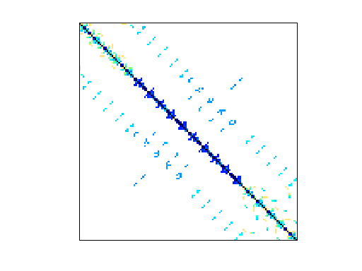
The two shallow_water* matrices arise from weather shallow water equations
(see http://www.icon.enes.org), from the Max-Plank Institute of Meteorology.
The problem gives rise to an automatic differentiation problem.  An iterative
solver is used for the larger problem, but a direct sovler is used for
finding the adjoints of a linear problem.  The velocity field is integrated
over a time loop with a semi-implicit method.  The implicit part leads to
a linear problem A*x=b, whose entries vary with time.  Two of these matrices
A are in this collection, with shallow_water1 at dtime=100 and shallow_water2
at dtime=200.  The nonzero patterns of the two matrices are the same, but
shallow_water1 is much slower.  The reason is that many denormals appear
during factorization, which greatly slows down the BLAS.  This can be solved
by compiling with gcc -ffast-math, to flush denormals to zero.
|